Creating a simple movement animation
example-1.RmdFirst, load the required packages for this example and the
moveVis example movement data:
move_data is a move2 data frame, containing
three individual tracks. moveVis works with such
move2 class objects. If your movement data are represented
by other classes, e.g. non-spatial data.frames, see
?move2::mt_as_move2 on how to coerce your data into
move2 class objects.
Let’s have a look at both timestamps and sampling rates of
move_data:
unique(mt_time(move_data))
mt_time_lags(move_data, unit = "min")
You can see that each track has a sampling rate of roughly 4 minutes.
However, sampling rates differ over time. Due to this, tracks do not
share unique timestamps. For animation, fixed regular frame times are
needed, regardless whether you want to animate a single track or
multiple tracks at once. Thus, we need to align move_data
in order to
- make all tracks share a unique time interval that can be matched by frame times
- make all tracks share a fixed sampling rate without gaps
To achieve the above, we need to apply interpolation. There are many
ways to spatio-temporally interpolate movement tracks. One basic
approach to this is linear referencing, as implemented via
align_move().
You can use align_move to align movement tracks to a fixed
uniform time scale of e.g. 4 minutes:
move_data <- align_move(move_data, res = units::set_units(4, "min"))Instead, you could apply your own functions for aligning your data, e.g. using more advanced interpolation methods.
Now, as movement tracks are aligned, we can pair them with a base map
to create frames that can be turned into an animation later on. You can
use your own base map imagery or choose from default map types provided
by the
basemaps
package. Here is a GIF of some example base maps you can use out of the
box:
You can display a list of all available maps like this:
# get a list of all available map_services and map_types
get_maptypes(as_df = TRUE)
#>          map_service                              map_type
#> 1                osm                               streets
#> 2                osm                            streets_de
#> 3                osm                           topographic
#> 4         osm_stamen                                 toner
#> 5         osm_stamen                              toner_bg
#> 6         osm_stamen                               terrain
#> 7         osm_stamen                            terrain_bg
#> 8         osm_stamen                            watercolor
#> 9         osm_stadia                        alidade_smooth
#> 10        osm_stadia                   alidade_smooth_dark
#> 11        osm_stadia                              outdoors
#> 12        osm_stadia                            osm_bright
#> 13 osm_thunderforest                                 cycle
#> 14 osm_thunderforest                             transport
#> 15 osm_thunderforest                             landscape
#> 16 osm_thunderforest                              outdoors
#> 17 osm_thunderforest                        transport_dark
#> 18 osm_thunderforest                                spinal
#> 19 osm_thunderforest                               pioneer
#> 20 osm_thunderforest                          mobile_atlas
#> 21 osm_thunderforest                         neighbourhood
#> 22 osm_thunderforest                                 atlas
#> 23             carto                                 light
#> 24             carto                       light_no_labels
#> 25             carto                     light_only_labels
#> 26             carto                                  dark
#> 27             carto                        dark_no_labels
#> 28             carto                      dark_only_labels
#> 29             carto                               voyager
#> 30             carto                     voyager_no_labels
#> 31             carto                   voyager_only_labels
#> 32             carto                  voyager_labels_under
#> 33            mapbox                               streets
#> 34            mapbox                              outdoors
#> 35            mapbox                                 light
#> 36            mapbox                                  dark
#> 37            mapbox                             satellite
#> 38            mapbox                                hybrid
#> 39            mapbox                               terrain
#> 40              esri                      natgeo_world_map
#> 41              esri                         usa_topo_maps
#> 42              esri                         world_imagery
#> 43              esri                    world_physical_map
#> 44              esri                   world_shaded_relief
#> 45              esri                      world_street_map
#> 46              esri                    world_terrain_base
#> 47              esri                        world_topo_map
#> 48              esri                  world_dark_gray_base
#> 49              esri             world_dark_gray_reference
#> 50              esri                 world_light_gray_base
#> 51              esri            world_light_gray_reference
#> 52              esri                  world_hillshade_dark
#> 53              esri                       world_hillshade
#> 54              esri                      world_ocean_base
#> 55              esri                 world_ocean_reference
#> 56              esri                     antarctic_imagery
#> 57              esri                        arctic_imagery
#> 58              esri                     arctic_ocean_base
#> 59              esri                arctic_ocean_reference
#> 60              esri world_boundaries_and_places_alternate
#> 61              esri           world_boundaries_and_places
#> 62              esri               world_reference_overlay
#> 63              esri                  world_transportation
#> 64              esri                delorme_world_base_map
#> 65              esri               world_navigation_charts
#> 66          maptiler                             aquarelle
#> 67          maptiler                        aquarelle_dark
#> 68          maptiler                       aquarelle_vivid
#> 69          maptiler                              backdrop
#> 70          maptiler                                 basic
#> 71          maptiler                                bright
#> 72          maptiler                               dataviz
#> 73          maptiler                             landscape
#> 74          maptiler                                 ocean
#> 75          maptiler                               outdoor
#> 76          maptiler                             satellite
#> 77          maptiler                               streets
#> 78          maptiler                                 toner
#> 79          maptiler                                  topo
#> 80          maptiler                                winter
Currently, you can use more than 75 types of maps, e.g. provided by
OpenStreetMap, Carto or Mapbox.
For some map services, you need a (free) map token for which you need an
account at the respective service (see
supported
maps<> for details).
In this example, we want to use the OpenStreetMap ‘topographic’
imagery with a transparency of 50% to standard with a fairly standard
type of map. To create a spatial frames from move_data
using a base map, we can use frames_spatial() like
this:
frames <- frames_spatial(move_data, path_colours = c("red", "green", "blue"),
                         map_service = "osm", map_type = "topographic", alpha = 0.5)
Instead of using path_colours, you can add a
colour column to your move2 object. This
allows you to colour your movement tracks as you want, e.g. not only by
individual track, but by behavioural segment, time, age, speed or
something different (see
?frames_spatial
for details).
Have a look at the newly created frames object. You can retrieve some information about the frames that you have just created and plot individual frames to get first impressions on how your animation will look like:
frames
#> moveVis frames (spatial), ≈ 7.52s at 25 fps using 188 frames
#> Temporal extent:  2018-05-15 07:03:59.636288 to 2018-05-15 19:31:59.636288
#> Spatial extent:   xmin: 990463.40648; ymin: 6060710.02464; xmax: 1001881.32133; ymax: 6069317.35905
#> CRS (projected):  WGS 84 / Pseudo-Mercator
#> Basemap:          'topographic' from 'osm'
#> Names:            'T932u', 'T342g', 'T246a'

length(frames) # number of frames
#> [1] 188
frames[[100]] # display one of the frames
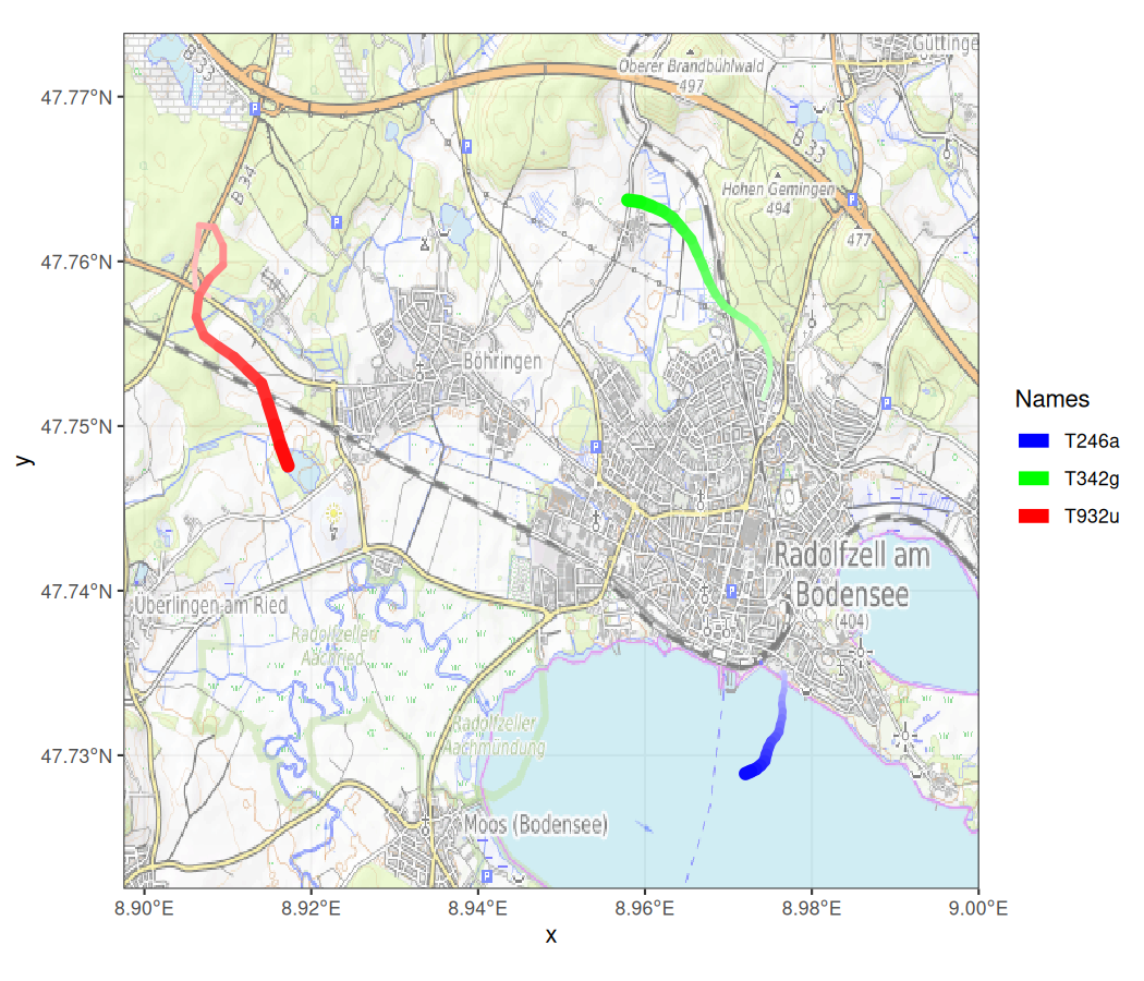
You can pass any moveVis frames object like the one we just created
to animate_frames(). This function will turn your frames
into an animation, written as a GIF image or a video file. For now, we
do not want to add
any customization to frames<> and just create a
GIF from it right away. If you are not sure, which output
formats can be used, run suggest_formats(). This function
returns a vector of file suffixes that can be created on your operating
system. For making a GIF from frames, just
run:
animate_frames(frames, out_file = "example_1.gif")
We have just used a classic OpenStreetMap map as base map. You can
try different map services and types (some of which are showcased as
visual
examples in the basemaps documentation):
frames <- frames_spatial(move_data, path_colours = c("red", "green", "blue"),
                         map_service = "carto", map_type = "light", map_res = 0.8)
frames[[100]] # display one of the frames
Like above, these frames can be put in motion using
animate_frames():
animate_frames(frames, out_file = "example_1b.gif")
That’s the basics of using moveVis! If you want to learn
more, take a look at
how
moveVis frames can be customized – either using the
moveVis add_ functions or by applying
ggplot2 code frame-by-frame.